

Quantifying Successful Possession (xPG)
/July 11, 2018
Cheuk Hei Ho (@tacticsplatform)
Expected Goals (xG) have become one of the essential tools in soccer analytics. It offers more insight than any model which uses raw shot numbers. xG uses location date to help differentiate the quality of shots that traditional methods fail to take into account. xG-based variants such as Expected Assists (xA) attempts to extend xG beyond the primary shooter to a passer or anyone who has contributed to the passing sequence leading to a shot. They aim to broaden the impact of xG.
But most xG-based methods still suffer one flaw: it describes a small portion of a soccer game. The typical soccer game in MLS averages about 15-20 shots per match. Organizing the game into possessions, sequences of uninterrupted – or if interrupted, the interruption lasts fewer than two seconds – action events (pass, dribble, shot…etc.), we will summarize the game into about 140 possession groups per game. Because most possessions can only create one shot every time, any xG-based method will overlook close to 90% of the possessions that don’t result in any shot. Therefore, any similar approach doesn’t provide a complete description of the game.
We need a method that isn’t dependent on shot creation. Some elements of soccer don’t present a clear and direct interaction with the shot, such as the tactical or the formational change. You can use the location of the players to decipher the shape of a team, but how do you measure the efficiency and the individual contribution of each position? To this end, we developed an xG-based score – Expected Possession Goal (xPG) – that is dependent on the location of the ball but not the shots creation.
Most possessions aim to move the ball within a shooting distance so that the player can score. xPG measures how a team uses its possession to achieve that goal. I first divide a soccer pitch into 162 zones. Each zone is assigned a zonal xG value by averaging all the shot xG values from the same zone from 2015 to 2018. I then group every match into the possession groups. Every action event, whether it is the shot or not, is given a zonal xG value based on which one of the 162 zones that it takes place. I summate all the zonal xG values within a possession to establish the xPG value for that possession. Any possession that reaches the shooting location, even if it doesn’t result in the shot, will have an xPG value. Every player will be given the same xPG if he has contributed to that possession.
In short, we group the game into the possessions, assign a value for each possession based on how successful it is, add them up and that value becomes the total xPG. Each player gets a share of the total xPG based on how many of those possessions he has contributed.
xPG measures how successfully the team and its players complete the possession.
We can use xPG to measure how different positions support the completion of possessions. I divide the players into six broad positions in this analysis:
1. Attacking central midfielder: an advanced central midfielder behind the forwards.
2. Central midfielder: any central midfielder except for the attacking central midfielder.
3. CB / center back: any central defender.
4. Forward: a lone striker or a forward in a two-striker’s formation.
5. Full back / Wing back: an outside defender on the flank or a wing back (an advanced full back) in a 3-5-2.
6. Wide attacker: a winger in a 4-4-2 or a 4-2-3-1, or an outside forward in a 4-3-3.
I exclude the keeper from this analysis. I have also isolated the attacking central midfielder since it has undergone numerous changes over the last decade. Its function has specialized and diversified in different systems.
I first characterize how each player or position and xPG interact in MLS this season. I assign two xPG measures, xPG contribution and xPG per minute for every player who has started for more than three games this season. xPG contribution is a relative measure to estimate the player’s contribution of the team’s completed possessions. It is calculated by dividing the player’s xPG over the team’s xPG for the time span the player has participated in the game. xPG per minute is an absolute measure by normalizing the player’s xPG with the minutes he has spent on the pitch in each game.

A summary plot of xPG contribution and xPG/minute. xPG contribution is a relative measure to estimate the player’s contribution of the team’s completed possessions. It is calculated by dividing the player’s xPG over the team’s xPG for the time span the player has participated in the game. xPG per minute is an absolute measure by normalizing the player’s xPG with the minutes he has spent on the pitch in each game. The correlation coefficient between xPG contribution and xPG is 0.85. Data accumulated until week 18 is used.
The attacking central midfielder has the highest xPG contribution, followed by the central midfielder, the wide attacker and the full back/wing back. The center back has the lowest successful possession contribution. Strikingly, most forwards have the lowest relative or absolute xPG. Why? If he is the most spatially advanced player, shouldn’t he also be the closest to the shooting distance where xPG tries to quantify, hence with a higher xPG? If we think about the problem more carefully, the forward’s low xPG is consistent with a principle of the game; the forward is the most capable player to convert the shot to the goal. A defending team should do everything it can to deter him from touching the ball at the shooting distance. Therefore, the forward should have low xPG; otherwise, you would be seeing a lot more goals in soccer.
xPG Detects Tactical Differences Between Different Teams
With a general idea of how different positions contribute to xPG league-wise, we can now examine how each role functions in different teams:

A summary of xPG contribution by the position for every team in MLS 2018. Only the positions which has been played fmore than five times this season is used.
This plot summarizes the xPG contribution of every position that has played more than five times for each team this season. Every team has a unique order of the xPG contributions from various positions, because of using different formations with a distinct tactics. Moreover, every team has a different pattern of how the xPG spreads over various positions. We can summarize the distributions of xPG with some simple parameters:

A scatterplot of the xPG contribution parameters for every team in MLS 2018. The mean and the median aim to seek the most representative xPG value for the team. The range measures the maximal difference while the standard deviation quantifies every difference between each position. Grey lines depict the average values of the two parameters on x- and y- axis.
The mean and the median aim to seek the most representative xPG value for the team. The median is more stable than the mean when dealing with extreme values such as those of FC Dallas. Bear in mind that the xPG contribution is a relative measure; a small value means a particular position(s) contributes a small fraction, not a small absolute amount, of the successful possessions. For examples, teams like New York Red Bulls and New England Revolution have two of the lowest median xPG contribution values in MLS, meaning that most positions in these teams contribute small fractions of the successful possessions. Their highest contributor, the attacking central midfielder, provides only about 50% of their successful possessions. If every position only contributes a small fraction, they must show little overlap, meaning that there is little cooperation between different positions when these teams attack: for instance, the central midfielder doesn’t always combine with the wide attacker, or the full back rarely connects the forwards. The style of these teams is consistent with their overall small xPGs; Red Bull New York and New England play a direct and chaotic brand of soccer. They don’t rely on the possession control. They want to play at a fast pace. If you're going to play fast, you can’t have every player touching the ball in every possession. You want to limit every possession into a handful of touches so that the ball can reach the shooting distance as quickly as possible.
The range measures the maximal difference while the standard deviation quantifies every difference between each position. Therefore, both values estimate how specialized the positions have evolved to help complete successful possessions. The range is easier to understand because it shows how much a team tends to specialize one role in xPG. For example, while every attacking central midfielder leads the xPG contribution, teams like FC Dallas and Portland Timbers deploy it as the sole position to orchestrate the attack with talented play-makers like Mauro Diaz, Sebastián Blanco, and Diego Valeri.
New York City is “a city of two tales” in xPG; New York Red Bulls and New York City FC have opposing styles regarding possession. In contrast to the furious and chaotic Red Bulls, New York City FC allocates many positions into the attack so that they can slowly build-up their offensive phase. However, they also have one designated offensive master in Maximiliano Moralez that is involved in close to 70% of the successful possessions while the Red Bull’s top offensive orchestrator, Alejandro “Kaku” Romero Gamarra doesn’t even hit half of their xPG.
While the attacking central midfielder and the central midfielder are the dominant positions in the successful possession for 18 MLS teams this season, five teams use the forward, the wide attacker, or the full back/wing back as their top xPG contributor. For example, Sporting Kansas City designates their full back/wing back as the primary offensive contributor. Breaking down the xPG contribution by the player level:
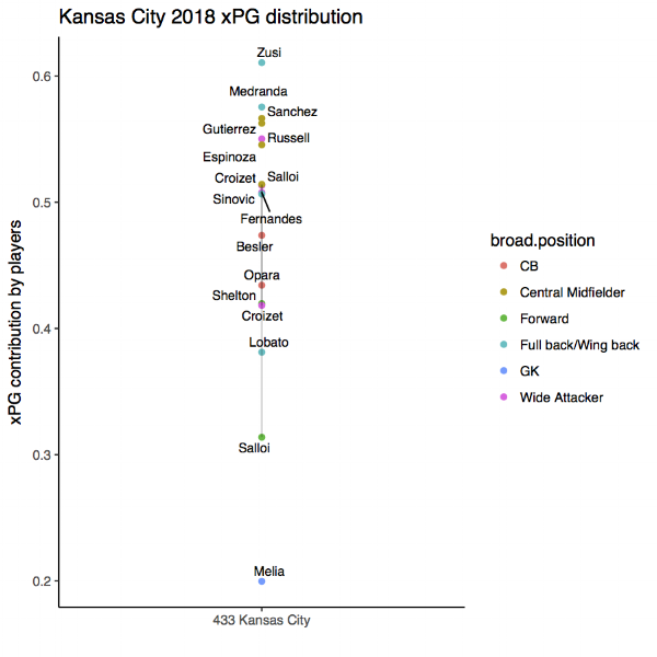
A summary of xPG contribution by position for Kansas City 2018. Only player in each position plays at least two times this season is included.
Graham Zusi and Jimmy Medranda are Kansas City’s top two xPG contributors followed by the central midfielders and then the wide attackers. They are the only team this season that puts so much offensive focus on their full back/wing back.
L.A. Galaxy is one of the two teams that uses their forward as the top xPG contributor. They use a 4-2-3-1 as the primary formation. Interestingly, other teams that use the 4-2-3-1 as the default shape, such as Columbus Crew and Minnesota United, usually deploy the central attacking midfielder as the crucial position in completing the possession. Comparing the xPG contribution by their player level:

A summary of xPG contribution by position for L.A. Galaxy 2018. Only player in each position plays at least two times this season is included.

A summary of xPG contribution by position for Columbus Crew 2018. Only player in each position plays at least two times this season is included.

A summary of xPG contribution by position for Minnesota United 2018. Only player in each position plays at least two times this season is included.
We find that L.A. Galaxy indeed use the attacking central midfielder as their top xPG contributor when they put Sebastian Lletget in that role. However, Lletget has only four starts in that positions and shares it with Romain Alessandrini, Jonathan dos Santos, and Giovani dos Santos. The most distinctive feature of the L.A.’s 4-2-3-1 is the xPG contribution by its star striker Zlatan Ibrahimovic; his xPG contribution is over 60%, at least 20% more than that of Columbus’ Gyasi Zardes or Minnesota United’s starter Christian Ramirez. Why? Zlatan is different from most strikers that he has excellent skill and can drop to the midfield and help to build up. In contrast, Zardes and Ramirez are typical strikers that focus on finishing the shot instead of building up the attack. The xPG data demonstrates those parts of their games.
xPG Detects Tactical Differences Between Different Formations of the Same Team
If we can compare two teams, we can also compare the change of xPG contribution between two lineups of the same team. Consider Chicago Fire’s formational changes:

A summary of xPG contribution by position for Chicago Fire 2018. Only player in each position plays at least two times this season is included. Grey lines depict the changes of xPG contribution by each player in different formations.
I will let you dwell on your favorite / most loathed team from all these graphs:


The Evolution of Positions and Formations
We can further develop the comparison of the xPG contributions across different formations ignoring the identity of the team so that we can examine how different positions evolve according to the formational change:

A summary of xPG contribution by the position for different formations in MLS 2018. Only the formation that has plays for more than five times this season is used.
This plot is similar to Fig.1, except that we separate the xPG contributions of the positions based on the 12 formations that have been used more than five times in MLS this season. Grouping the position based on the formation still preserves the trend we have seen; the attacking midfielder is the top xPG contributor while the wide attacker and the central midfielders are close behind it. The center back is again the lowest xPG contribution. But we also see some changes: the full back/the wing back and the forward are not the xPG priority in any formation, meaning that the role of Zusi or Ibrahimovic in Kansas City and L.A. must be player- and team- specific.
The best way to test the accuracy of our method is to compare the result with a gold standard. Such a standard doesn't exist, so we need to find an alternative. We need to check whether our result is consistent with the similarity of the formations based on what we know about them. We can check if two similar formations have a similar order of the xPG contributions between different positions. Two formations, the 3-5-2, and the 5-3-2, closely resemble each other; they both use three center backs, three central midfielders, two forwards, and two wing backs. The only difference between them is the position of the wing backs: they stay closer to the center backs in the 5-3-2 than they do in the 3-5-2. Our xPG contribution ordering finds that the only difference between them is the order of the forward and the wing back: the wing back has a higher xPG contribution than the forward in the 3-5-2. This result makes sense, because the wing back has a more advanced position in the 3-5-2 than in the 5-3-2. But we also have a discrepancy that the defensive 5-3-2 has a higher xPG contribution than that of the 3-5-2. Bear in mind the xPG contribution is a relative measure but not an absolute measure. The absolute measure of xPG, the xPG per minute, shows that both formations produce close to 10 xPG per 96 minutes (10.08 in the 3-5-2 vs. 9.89 xPG in the 5-3-2). xPG also only measures the offensive but not the defensive contribution, so the defensive strength of the formation may not show up in any xPG parameter. Therefore, our method can detect the subtle difference of the possession completion of various positions in similar formations.
The formations change according to the strategic shift and player development. A modern tactical trend is the specialization of the player’s role; we used to have three roles: the defender, the midfielder and the forward. Now we have the evolution of the wing back from the full back, or the split of the midfielder into the defensive and attacking one. The same movement has repeated in MLS; ten years ago every team played a primary 4-4-2 formation. This season, more than a dozen formations have been deployed. Almost every 4-4-2 variant such as 4-4-1-1 and the 4-2-3-1 have been used more than five times. The introduction of the attacking central midfielder changes how the 4-4-2 variants attack, as shown by the increased range and standard deviation of 4-4-1-1 / 4-2-3-1 vs. 4-4-2:

A summary of xPG contribution by the position for different formations in MLS 2018. Only the formation that has plays for more than five times this season is used.

A scatterplot of the xPG per 96 minutes and xPG contribution for every qualified formation in MLS 2018. Grey lines depict the average values of the two parameters on x- and y- axis.
For example, a 4-3-1-2 uses the attacking central midfielder but its xPG / 96 minutes, an absolute measure of the offensive performance, is lower than the average of all of the qualified formations. Comparing to other formation featuring the attacking central midfielder, the 4-3-1-2 does not support its attack with the wing back or the wide attacker. The lack of width in attack is a trade-off of the 4-3-1-2; it is another 4-4-2’s variant with the wide-midfielders shifting toward the center to bolster the control of the middle area. These midfielders take on the #8 box-to-box role to strength both the offensive and the defensive phases. The full back has to carry the offensive load on the flank. The failure to boost its offensive contribution from this position may explain 4-3-1-2’s mediocre offensive output: the withdrawn position of the full back compared to that of the wing back may increase the physical burden for the former and prevents it from engaging in the attack.
Nevertheless, a designation of the attacking central midfielder benefits the offensive performance of most formations. It also explains Atlanta United’s formation’s choice; the strength of the 3-5-2 is its focus in the center. A total of six players position in the middle of the first two lines. Although this arrangement promotes the control of the possession, its xPG output is low. By deploying Miguel Almiron as a specific offensive orchestrator in a 3-4-1-2, Gerardo Martino achieves an outstanding offensive prowess while retaining the advantage of the 3-5-2.
The Limitations of xPG
Because xPG measures how successfullu the team and its players complete the possession, we can use it to determine how the role of individual position evolves in different formations. But it has its limitations. For example, it does not attempt to measure how effectively a team can convert the successful possession into the shot or the goal. We need to connect xPG with any or all of the xG variants. At this stage, xPG doesn’t provide a complete description of the game.
But no one single measure does; think about a final score of the game. It summarizes the outcome of the match with two numbers but discards the spatial, the temporal, or the individual player’s information. xG or its variants ignore any event that doesn’t lead to a shot, or the pass map/network collapses the spatial data into a dozen of spots by multiple orders. The only summary that retains all the data of the game is the game itself. Between the game and the score, many different summaries should be available so we can organize and analyze the game to approach the complete description.