

Expected Goals 3.0 Methodology
/By Matthias Kullowatz (@mattyanselmo)
Michael Bertin of Deadspin recently critiqued the expected goals craze that is rushing through advanced soccer metrics. He specifically noted that so many expected goals models are currently proprietary, hidden inside of black boxes. We here at ASA have sought to be as transparent as possible, and so we have published our logistic* expected goals models in the Explanation section of our xGoals 3.0 tab above.
Many of the variables in the model are intuitive. The distance from the shooter to the goal obviously affects the difficulty of the shot, as well as the angle from which the shot was taken. Shots off corner kicks have a lower chance of going in--once controlled for shot location, angle, body part, and other factors--because the box is packed. Fastbreak shots off through balls have a high chance of going in because the shooter often has time and space. The variables in the basic shooter/team model include: distance, goal mouth available, whether the shot was headed, whether the shot came off a cross or through ball, and whether the shot came from any one of the various patterns of play including corner kicks, direct free kicks, indirect free kicks, fastbreaks, or penalties. The "regular" pattern of play is included in the intercept term.

A recent change we have made is substituting a log-Distance variable into the model for what was just a linear Distance variable. This idea was admittedly inspired by Bertin. Using log-Distance will change some of the output on the blog because the results of extremely close and extremely distant shots were not being as accurately predicted as they are now. Justification for this change can be seen in the graph to the right. The trend is that of a (negative) log function rather than a linear function. Note the spike around 13 yards. These are penalties, and as you can see, our model's calibration is off a bit. Penalties average 13 yards in distance in our data set, though this will not effect the utility of the model because distances are relative.

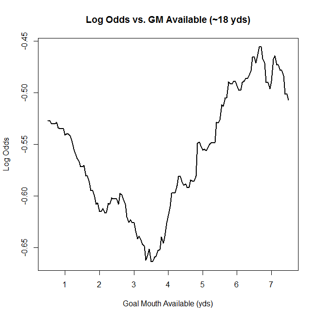
I have also updated how the model treats the width of the goal mouth available to the shooter. From straight on, a shooter has eight yards from left post to right post. But as his angle gets worse, that width available can shrink considerably. To appropriately model the effect of goal mouth availability, I used a quadratic function, which is justified to the right. The plot shows how the log odds of a goal change due to angle, with diminishing returns for better angles. Here, shot distance is frozen between 9 and 15 yards.
Additional Keeper Model Variables
The height of the shot in the goal mouth is also important. Players aim both low and high to try and beat the keeper, and justification for that strategy is borne out beautifully in the graph shown to the right. The log odds of a goal increase the further the shot height is from a comfortable 3.5 feet. The decline in log odds between about 6.5 and 8 feet is a bit perplexing, though. I controlled for distance on this graph, but not other factors. It turns out that 21 percent of all shots in the upper portion of the goal mouth were headed, versus just 14 percent of shots below that zone. This surely plays a role in the strange behavior between heights of 6.5 and 8 feet, and we have controlled for headed shots in the model. Here, shot distance is frozen between 15 and 21 yards.
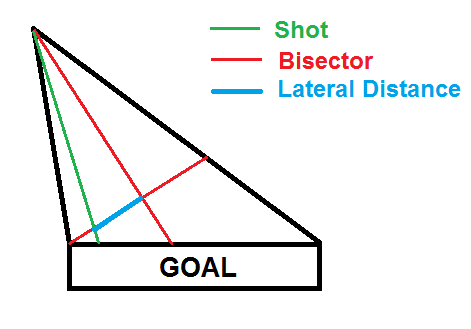
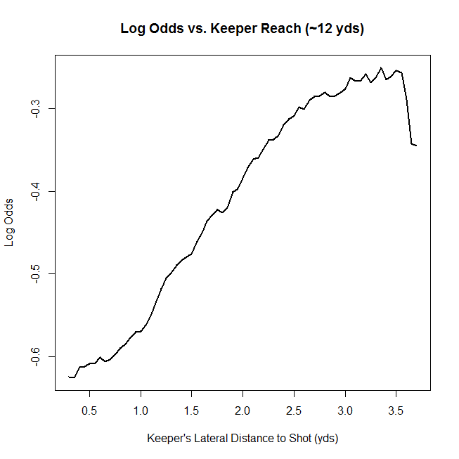
The last variable I'm going to justify is the linear version of the lateral distance a keeper had to move to make a save. This was the hardest part of the model mathematically, as it required some tricky analytic geometry and some basic assumptions about keeper positioning that aren't always true. Basically, we assume that keepers position themselves along the angle bisector of the two rays that extend from the shot to both posts. If they don't, then they should (usually). The lateral distance to the shot is then measured along a line that goes through the near post, perpendicular to the angle bisector. The geometry, as well as justification for the linear term in the model, are shown below. Again, there is strange behavior in the log odds when the lateral distance is between 3.5 and 4. The is because very few shots are taken from straight on, and thus the sample size is incredibly small and subject to weird fluctuation. Here, shot distance is frozen between 9 and 15 yards.
For logistic models (and many other general linearized models and non-linear models), the R-square value is not a particularly intuitive value. I hope the p-values in the models above, in addition to the graphs and basic logic about soccer, help to justify our Expected Goals 3.0 model.
*Logistic models use a log odds response instead of a probability. This is because linear models by themselves could potentially arrive at probabilities above 1.0 or below 0.0. Log odds are the natural logarithm of the ratio of probability of success "p" to probability of failure "1 - p," or ln[p/(1-p)].